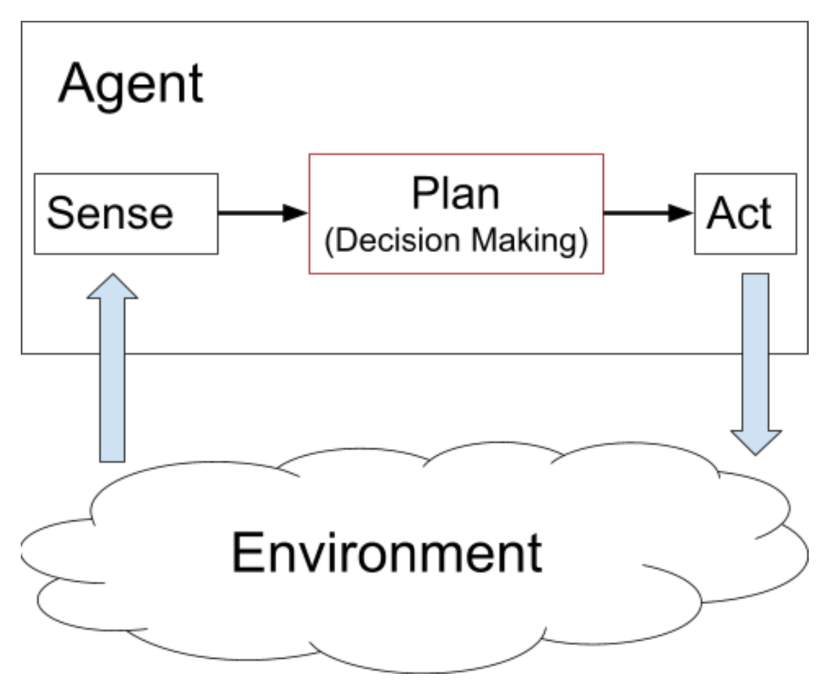
Autonomously controlling a car is challenging and requires solving a number of subproblems. If perception, which understands information from sensors, corresponds to the eyes or our system while control, which turns the wheel and adjusts the velocity, corresponds to the body having a physical impact on the car, then decision making is the brain. It must connect what is perceived with how the car is controlled.
In this blog post, we discuss the challenges in designing the brain of an autonomous car that can drive safely in a variety of situations. First, we introduce the scope and motivation for decision making before presenting how it is currently implemented in Autoware. We then talk about the trends observed in recent autonomous driving conferences and briefly introduce a few works that propose interesting new directions of research.
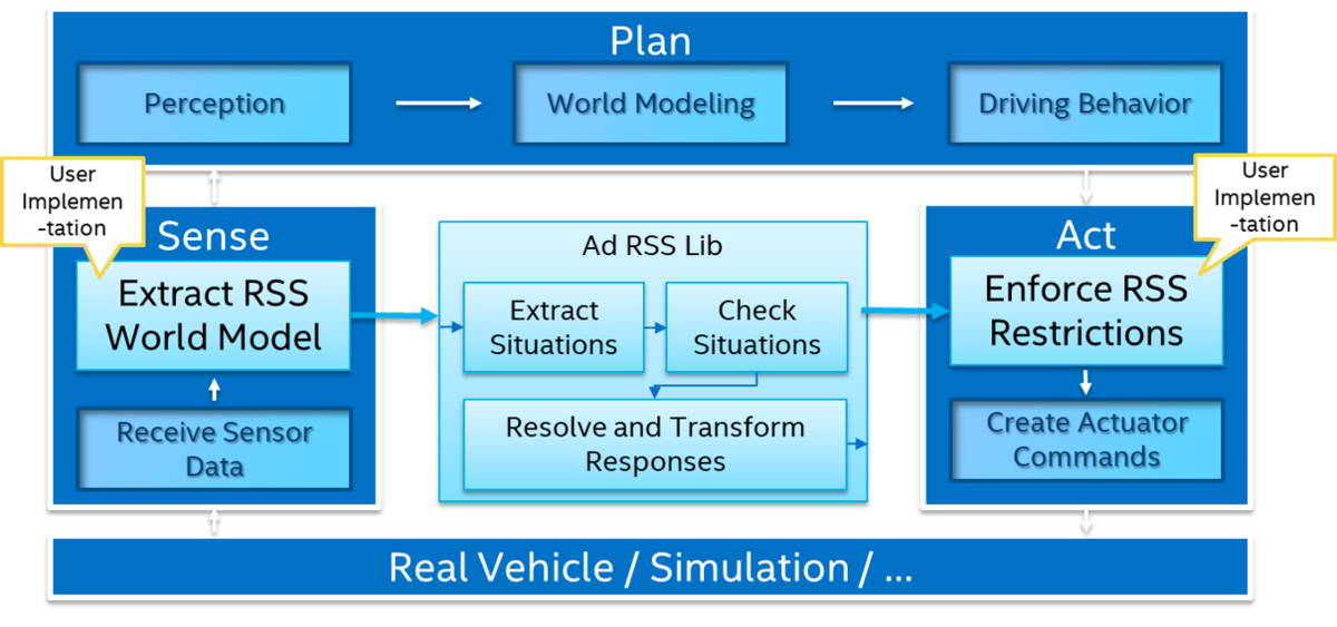
Figure 1 - Typical sense-plan-act paradigm for autonomous agents
By the way, at Tier Ⅳ, we are looking for various engineers and researchers to ensure the safety and security of autonomous driving and to realise sharing technology for safe intelligent vehicles. Anyone who is interested in joining us, please contact us from the web page below.
We spend our life making decisions, carefully weighing the pros and cons of multiple options before choosing the one we deem best. Some decisions are easy to make, while others can involve more parameters than can be considered by a single human. Many works in artificial intelligence are concerned with such difficult problems. From deciding the best path in a graph, like the famous Dijkstra or A* algorithms, to finding the best sequence of actions for an autonomous robot.
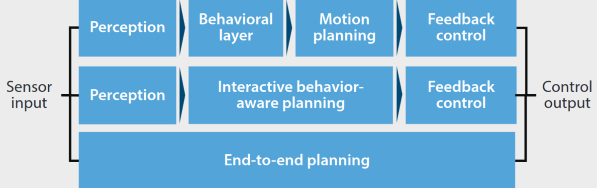
For autonomous vehicles, decision making usually deals with high level decisions and can also be called behavior planning, high-level planning, or tactical decision making. These high level decisions will then be used by a motion planner to create the trajectory to be executed by the controller. Other approaches consider planning as a whole, directly outputting the trajectory to execute. Finally, end-to-end approaches attempt to perform all functions in a single module by using machine learning techniques trained directly on sensor inputs. While planning is one of the functions handled by end-to-end techniques, we will not discuss them in this blog post as they tend to make decision making indistinguishable from perception and control.
The common challenge unique to decision making systems comes from the open-endedness of the problem, even for humans. For perception, a human can easily identify the different objects in an image. For control, a human can follow a trajectory without too many issues. But for decision making, two drivers might make very different decisions in the same situation and it is almost never clear what is the best decision at any given time. The goals of an autonomous car at least seem clear: reach the destination, avoid collisions, respect the regulations, and offer a comfortable ride. The challenge then comes from finding decisions that best comply with these goals. The famous “freezing robot problem” illustrates this well: once a situation becomes too complex, not doing anything becomes the only safe decision to make and the robot “freezes”. Similarly, the best way for a car to avoid collisions is not to drive. A decision system must thus often deal with conflicting goals. Challenges also arise from uncertainties in the perception and in the other agents. Sensors are not perfect and perception systems can make mistakes, which needs to be carefully taken into account as making decisions based on wrong information can have catastrophic consequences. Moreover, cars or pedestrians around the autonomous vehicle can act in unpredictable ways, adding to the uncertainty. Dedicated prediction modules are sometimes used and focus on generating predictions for other agents. The final challenge we want to mention here comes from dealing with occluded space. It is common while driving not to be able to perfectly perceive the space around the car, especially in urban areas. We might be navigating small streets with sharp corners or obstacles might be blocking the view (parked trucks for example), potentially hiding an incoming vehicle.
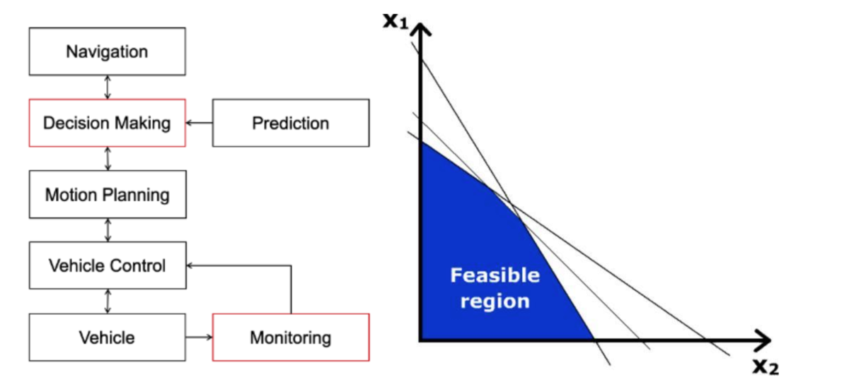
Figure 2 - Standard autonomous driving architecture
Schwarting, Wilko, Javier Alonso-Mora, and Daniela Rus. "Planning and decision-making for autonomous vehicles." Annual Review of Control, Robotics, and Autonomous Systems (2018)
To summarize, we are concerned with the problem of making decisions on the actions of the car based on perceptions from sensors and the main challenging points are:
conflicting goals that require trade-offs;
uncertainties from perception, localization, and from the other agents;
occluded parts of the environment.
In the rest of this post we will try to introduce methods to make decisions and to tackle the aforementioned challenges.
Decision Making in Autoware
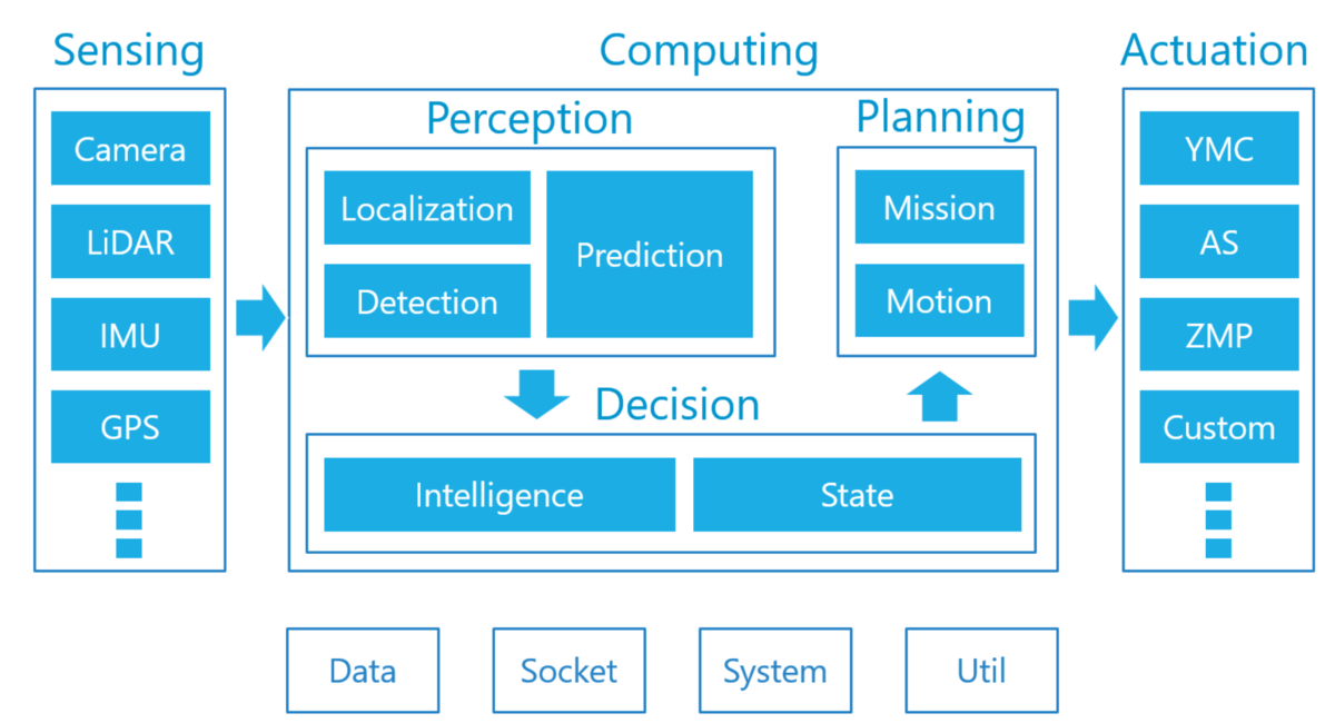
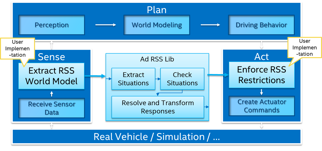
Figure 3 - Autoware architecture
Autoware is an open source project providing a full stack software platform for autonomous driving including modules for perception, control and decision making. In the spirit of open source, its architecture is made to have each function be an independent module, making it easy to add, remove, or modify functionalities based on everyone’s own needs.
In this architecture, decision making occurs at two stages. At the Planning stage, various planning algorithms such as A* or the Model Predictive Control are used to plan and modify trajectories. Before that, at the Decision stage, the output of perception modules is used to select which planning algorithms to use for the current situation. For example, it can be decided that the car should perform a parking maneuver, in which case a specific parking module will be used (Motion Planning Under Various Constraints - Autonomous Parking Case - Tier IV Tech Blog). This Decision stage is implemented using a Finite State Machine (FSM), a common model used in rule-based systems. A state machine is basically a graph representing possible states of the system as nodes and the conditions to transition between these states as edges. State machines are easily designed by humans and offer decisions that are easy to understand and explain, which is very desirable in autonomous driving systems.
While the decision and planning modules of Autoware offer state-of-the-art driving in nominal cases, they are not well suited to deal with uncertainties or occluded space. There are no classical approaches to deal with these challenges but they are studied by a lot of ongoing research, which we will discuss in the next part.
Deep Reinforcement Learning (DRL) is an application of deep neural networks to the Reinforcement Learning framework where the goal is to learn what action works best at each state of the system, corresponding to a policy Π(s) = a representing the decision a to take at state s. This usually requires learning a function Q(s,a) which estimates the reward we can obtain when performing action a at state s. In simple environments, this function can be computed by completely exploring the search space but when the state and action spaces become too large, like in autonomous driving problems, more advanced techniques must be used. DRL leverages the power of deep neural networks to approximate the function Q(s,a), allowing the use of RL in very complex situations. This requires training on a large number of example situations, which are usually obtained using a simulator. The biggest issue with using these techniques on real vehicles is the difficulty to guarantee the safety of the resulting policy Π(s). With large state spaces, it is difficult to ensure that there does not exist a state where the policy will take an unsafe action.
Mixed-Integer Programming (MIP) is an optimization technique which maximizes a linear function of variables that are under some constraints. Some of these variables must be restricted to integer values (e.g., 0 or 1) and can be used to represent decisions (e.g., whether a lane change is performed or not). The problem of an autonomous vehicle following a route can be represented with MIP by including considerations like collisions and rules of the road as constraints. Using commonly available solvers, the problem can then be solved for an optimal solution, corresponding to the best values to assign to the variables while satisfying the constraints. Many approaches applying MIP to autonomous driving have been proposed and while they can solve many complex situations, they cannot handle uncertain or partial information and require accurate models of the agents and of the environment, making them difficult to apply to real-life situations.
Monte-Carlo Tree Search (MCTS) is an algorithm from game-theory which is used to model multiplayer games. It is most famous for being used in AlphaGo, the first program able to defeat a human professional at the game of Go. The MCTS algorithm assumes a turn-based game where agents act in succession and builds a tree where each node is a state and where a child is the expected result from an action. If complete, the tree represents the whole space of possible future states of the game. Because building a complete tree is impossible for most real problems, algorithms use trial-and-error, similar to reinforcement learning, to perform sequences of actions before simulating the resulting outcome. This approach has the advantage of considering the actions of other agents in relation to our own decisions, making it useful in collaborative scenarios where the autonomous vehicle must negotiate with other vehicles (e.g., in highway merges). The main issue with MCTS is their computational complexity. As the tree must be sufficiently explored in order to confidently choose actions, it can be hard to use in real-time situations.
In the next section, we will present some recent works related to each of these trends.
Interesting Works
Graph Neural Networks and Reinforcement Learning for Behavior Generation in Semantic Environments
Patrick Hart(1) and Alois Knoll(2)
1- fortiss GmbH, An-Institut Technische Universität München, Munich, Germany.
2- Chair of Robotics, Artificial Intelligence and Real-time Systems, Technische Universität München, Munich, Germany.
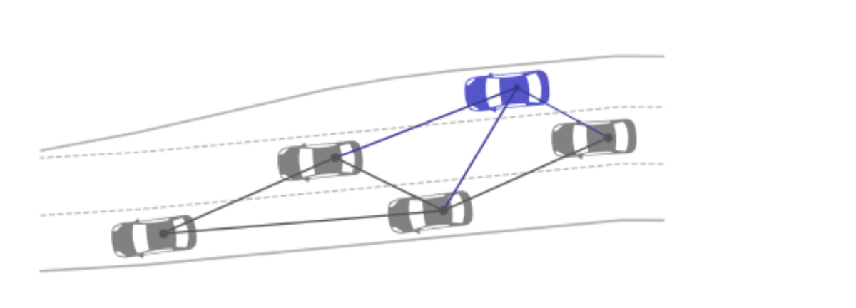
Figure 4 - Vehicles of a scene represented as a graph
An issue with reinforcement learning is that their input is usually a vector of fixed size. This causes issues when tackling situations with varying numbers of other agents. This paper proposes to use Graphic Neural Networks (GNNs) to learn the policy of a reinforcement learning problem. GNNs are a neural network architecture that uses graphs as inputs instead of vectors, offering a solution that is more flexible and more general than previous works.
The graph used in this paper represents vehicles with the nodes containing state information (coordinates and velocities) and the edges containing the distance between two vehicles. Experiments on a highway lane change scenario are used to compare the use of GNNs against the use of traditional neural networks. It shows that while results are similar in situations close to the ones used at training time, the use of GNNs generalizes much better to variations in the input without a significant loss of performance.
Autonomous Vehicle Decision-Making and Monitoring based on Signal Temporal Logic and Mixed-Integer Programming
Yunus Emre Sahin, Rien Quirynen, and Stefano Di Cairano
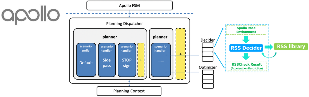
Figure 5 - (a) modules targeted by this work (b) illustration of the MIP solution space
This work uses Mixed-Integer Programming to represent the problem of finding intermediate waypoints along a given route. The interesting parts of this work are its use of Signal Temporal Logic (STL) to represent some of the constraints, and a monitoring system that can identify if the environment changes in ways that deviate from the models used.
Temporal Logic is a language used to write rules which include some time information. In this work for example, intersections are regulated by a first-in-first-out rule, which in STL is written as , which means “the car must not be at the intersection until it is clear”. The paper proposes an efficient way to encode STL rules as constraints, reducing the solution space of the problem (like in Figure 5b) and ensuring that they are satisfied by the solution of the MIP.
The paper tackles a simulated scenario with intersections and curved roads and shows that their solution can navigate a number of situations in real-time. They also show that their monitoring system can correctly detect unexpected changes in the environment, for example when another vehicle suddenly brakes. It is then possible to fall back to another algorithm or to solve the MIP problem again but with the new information added. This alleviates the main issue of MIP which is to depend on very good models of the environment as it is now possible to detect when these models make a mistake.
Accelerating Cooperative Planning for Automated Vehicles with Learned Heuristics and Monte Carlo Tree Search
Karl Kurzer(1), Marcus Fechner(1), and J. Marius Zöllner(1,2)
1- Karlsruhe Institute of Technology, Karlsruhe, Germany
2- FZI Research Center for Information Technology, Karlsruhe, Germany
As discussed in the previous section, MCTS are great to model interactions with other agents but are very hard to sufficiently explore. In order to make exploring the tree more efficient, this paper learns Gaussian mixture models that associate each state (i.e., node of the MCTS) some probabilities on the action space. These probabilities are used to guide the exploration of the tree.
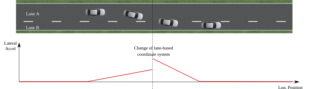
A Gaussian mixture is a combination of several Gaussian probability distributions, allowing multiple peaks with different means and covariances (Figure 6b). In this paper, the actions modeled by these probabilities are pairs of changes in longitudinal velocity and in lateral position. This means that for a given state, the mixture must contain as many peaks as there are possible maneuvers such that their mean will correspond to the typical trajectory for that maneuver. On the highway for example, mixtures with 2 components can be used to learn the 2 typical maneuvers of keeping or changing lanes (Figure 6a).
This technique is interesting to make the exploration faster but the experiments of the paper do not show any performance improvements once enough exploring time is given. Having to fix the number of components can also be an issue when trying to generalize to various situations.
Conclusion
Decision making for autonomous driving remains a very important topic of research with many exciting directions currently being investigated.
Researchers and engineers at Tier IV are working to bring the results of this progress to Autoware as well as to develop new techniques to help make autonomous driving safer and smarter.
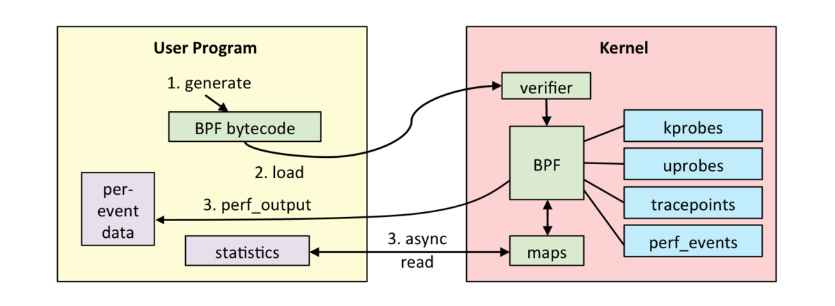
# Get offset address of the specified function
$ nm -D  /path/to/binary_file | c++filt | grep <function_name>
# Get the mangled function name
$ nm -D /path/to/binary_file | grep <offset>
Autonomous vehicles (robots, agents) are requested to move around in an environment, executing complex, safe maneuvers without human interference and to make thousands of decisions in a split second. How can we endow autonomous vehicles with these properties?
By the way, at Tier Ⅳ, we are looking for various engineers and researchers to ensure the safety and security of autonomous driving and to realise sharing technology for safe intelligent vehicles. Anyone who is interested in joining us, please contact us from the web page below.
Then, the key to answering this question is “Motion Planning”. Autonomous vehicles should be able to quickly generate motion plans and choose the best among many or the optimal plan defined by some optimization criteria.
Motion planning modules for autonomous driving might serve for three different objectives [1]:
Producing a trajectory to track,
Producing a path to follow,
Producing a path and trajectory with a definite final configuration.
In a trajectory tracking task, agents execute time-stamped commands to satisfy the spatial coordinates with the prescribed velocities. In the path tracking, only positions are tracked.
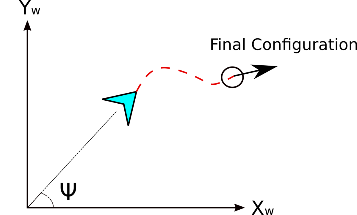
Vehicle motion is formally defined using a couple of differential equations. These differential equations propagate the state variables such as velocities (Longitudinal and lateral velocities; Vx, Vyand Heading Rate ) in the chosen coordinate system. The resultant integral curves define the configuration space of the robots (see Figure 1.). If we are controlling robots by velocities, the motion equations are called kinematic model equations.
Figure 1. Configuration space (x, y and heading rate) for a car-like robot motion
The most difficult task in the objectives list is the last one: to generate a trajectory or a path while satisfying the endpoint configuration. We are familiar with this kind of planning tasks from our daily life. You can probably remember how frustrating it was to park a vehicle within a parking slot the first time and execute a couple of maneuvers without hitting the cars or walls around (Figure 2).
Figure 2. Parallel parking
Why is planning with the endpoint configuration a difficult task even for cases without any obstacle in the environment?
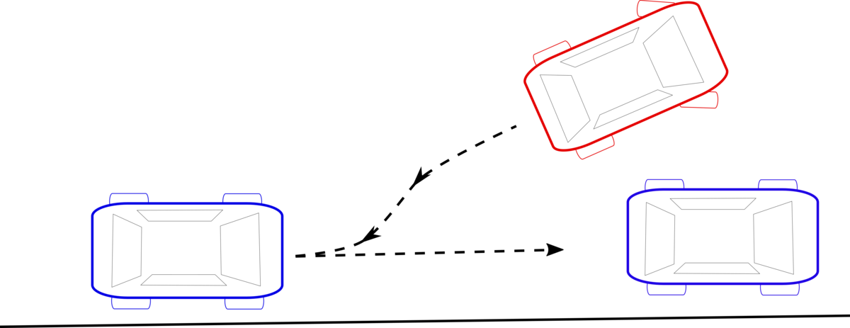
When considering the parking maneuver, notice that a car can only move forward-backward directions. If we also turn the steering wheel, the vehicle follows a circular path. Cars cannot move in their sideway direction as it is impossible due to the fixed rear wheel orientation. On the other hand, while executing a parking maneuver, we need to be able to move the car in the sideway directions to properly park the vehicle. That is why we drive the car, backward-forward and steer to move the car’s position in parallel to the starting position (Figure 3).
Figure 3. To move the car in the sideway direction parallel to the starting configuration, we need at least two maneuvers.
In physics, the prohibited sideway directions mean zero velocity in these directions. Although there are no environmental obstacles or physical constraints in these directions, the velocity is constrained to be zero. We can not integrate these velocities to convert them to path constraints which are relatively simpler to deal with. These velocity constraints are called "non-holonomic" motion constraints.
Since we have three motion direction (x, y and heading angle) and two controls (Speed V and steering δ), these kinds of systems are called under-actuated. Non-holonomic systems are in general under-actuated. Finding a path given two configuration positions respecting the velocity constraint is difficult due to the missing control direction.
Almost five decades of research effort has been put into finding a solution for non-holonomic motion planning. There has been no general solution proposed so far to the problem. Although it is possible to move a car position in parallel with a couple of maneuvers, such as zigzagging (Figure 3), the resultant paths and trajectories are discontinuous and generally have some cusp and breakpoints. This makes the solutions more difficult to find smooth trajectories mathematically. The nonholonomic motion planning problem becomes even more difficult when there are constraints in the environment (such as parking a vehicle in between the other vehicles). What is more, the motion equations are usually nonlinear and nonlinear differential equations do not have a direct solution except in a few cases.
In the robotics literature, approximate solutions have been proposed. These solutions are based on the notion of local controllability and the geometry of the configuration space. In principle, a global motion between two endpoints is divided into small motion trajectories. The small motion intervals are then connected using various algorithms.
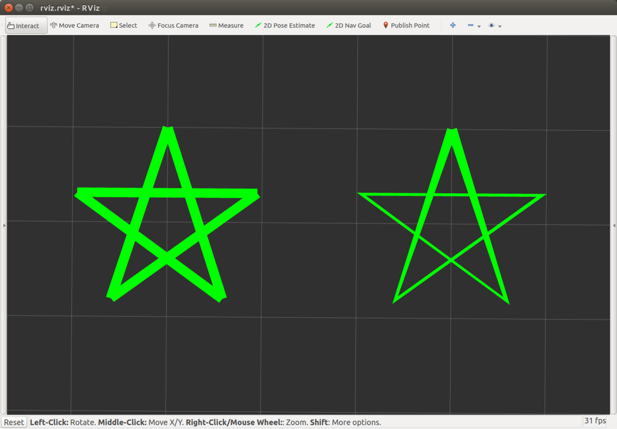
When there are no obstacles in the environment, we can use Reed & Shepp Curves (R&S Curves) to generate a direct path given two endpoints [2]. The R&S curves fit a path for the given endpoint configurations using some motion primitives; Straight (Backward-Forward), Left - Right Turns (Forward-Backward).
A couple of examples of R&S curves are shown in the following figures [3].
Figure 4. Reeds and Shepp curves for two different endpoint conditions.
Even though the R&S curves produce time-optimal and pleasing curves, they cannot provide a solution when there are environmental constraints. Their use is limited to unconstrained cases.
The most recent literature focuses on two-staged nonlinear optimization-based solutions for constrained environments. Nonlinear Optimization (Nonlinear Programming techniques - NLP) can deal with nonlinear motion equations and constraints. However, the nonlinear optimization methods require a good feasible solution to start with. This difficulty is what diversifies the proposals in the literature. We can list these methods under four categories. These are;
Optimization-based (bi-level or multi-staged optimization)
The proposed algorithms have advantages and disadvantages relative to each other. The common theme of these algorithms is having a two-stage solution that contributes to the implementation complexity.
At Tier IV, we have proposed a new algorithm for autonomous vehicle parking maneuvers inspired by an optimization method trending in the aerospace industry for designing spacecraft trajectories. The Successive Convexification Algorithm (SCvx) is capable of returning a feasible trajectory under a wide range of initial conditions, removing the need for a two stage approach, and has been proven to converge to the solution of the original nonlinear problem without compromising accuracy. In the next section, we explain what kind of problems we can encounter in the numerical solution of optimization problems, and how the successive convexification methods offer a solution to constrained nonholonomic motion planning.
Solving Nonlinear Problems by Successive Convexification Algorithms
Apart from a very demanding feasible initial solution in nonlinear programs, a design engineer can experience infeasible solution error messages raised by the solvers used in the numerical problem although the original problem is feasible. This kind of infeasibility is called artificial infeasibility. Solvers in numerical optimization have a mechanism to check beforehand whether the problem is feasible or not. The cause of infeasibility can be attributed to the results of implicit or explicit unrealistic linearization.
Furthermore, linear functions might not have a lower bound in the search space. This could be another reason for the solvers to halt. The lack of a lower bound in a minimization problem is called “artificial unboundedness” [see 3, 4, 5 and references therein].
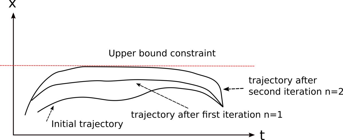
The SCvx algorithm is a kind of sequential quadratic optimization. In the sequential solutions, the nonlinear motion and constraint equations are linearized starting from an initial trajectory. Almost in all mathematical problems, one of the best strategies for the solution is to convert complex problems into a series of linear problems.
The solution of a linear problem yields a feasible trajectory which is then used as an initial trajectory for the next solution (Figure 5).
Figure 5. A nonlinear trajectory can be approximated by linear sub-problems which can be solved iteratively.
The SCvx algorithm operates in the same manner with two additional mechanisms to prevent artificial infeasibility and artificial unboundedness error messages.
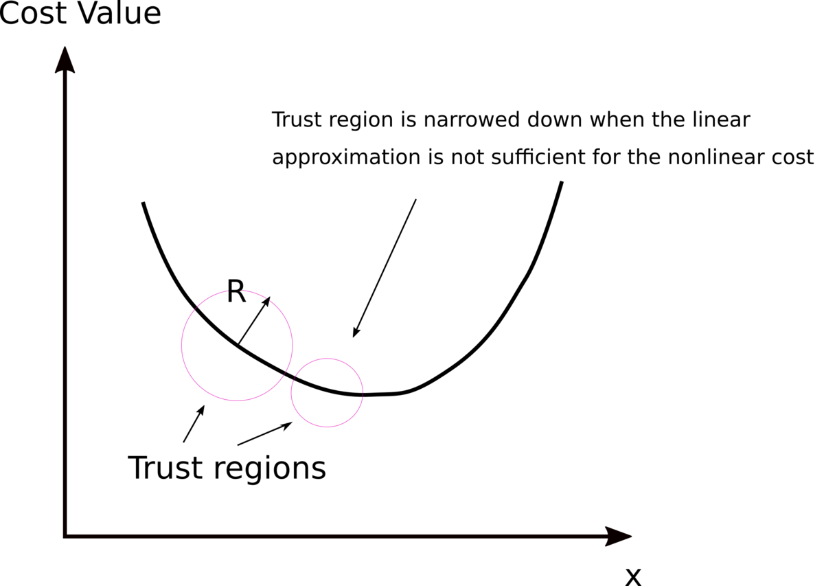
The artificial unboundedness problem is addressed by introducing a trust region that restricts the search space (Figure 6). The radius of the thrust region is adjusted by checking if our linearization reasonably approximates the nonlinear cost. If the linearization approximates the nonlinearity well enough, the radius of the trust region is increased, and vice versa.
Figure 6. Trust regions are used to restrict the search space of the optimization algorithm. The minimum or maximum is sought within the circles specified by the trust region radius.
The artificial infeasibility problem is addressed by adding a virtual force pushing all the infeasible states into a feasible region. However, the amount of virtual force we apply is penalized in the cost function with a very high weighting factor (i.e 1e5). One of the objectives is to make the contribution of the virtual force to the cost zero in the optimization.
These two additional mechanisms to prevent artificial infeasibility and unboundedness prevent the solvers from stopping due to the numerical problems and allow the solvers to seek the solution. The SCvx algorithms have been proved to converge to the original nonlinear solution. When a solution of the linear counterpart of a nonlinear problem is equivalent, the solution is called lossless (no feasible region is removed from the problem, [5]).
How Does the Successive Convexification Algorithm (SCvx) Help in Solving the Autonomous Parking (Nonholonomic Motion Planning) Problem?
So far, we alluded that the SCvx algorithm could give us a solution for a nonlinear optimization problem by solving sequential linear sub-problems. We also emphasised a virtual force that pushes infeasible states into the feasible state-space regions, and later on, this force is driven to zero. These two properties eliminate the need for a feasible initial trajectory, therefore reducing the two-stage solutions into one. The SCvx algorithm does not require an initial feasible trajectory. This is a highly desirable property since it is generally a hard problem to come with an initial trajectory in nonlinear optimization problems.
Although we are now closer to the solution for an autonomous parking problem, we need to overcome the other continuity issues afflicted. When we have a look at the R&S curves, point-to-point trajectories might require forward-backward - full stop motion. The vehicle moves a bit forward, stops fully, makes a full steering turn and moves back. There are both input and output discontinuities. The solvers and optimization algorithms operate on the continuity assumption. The second issue is the discontinuities in the environmental constraints.
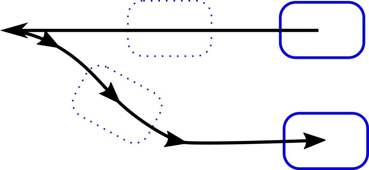
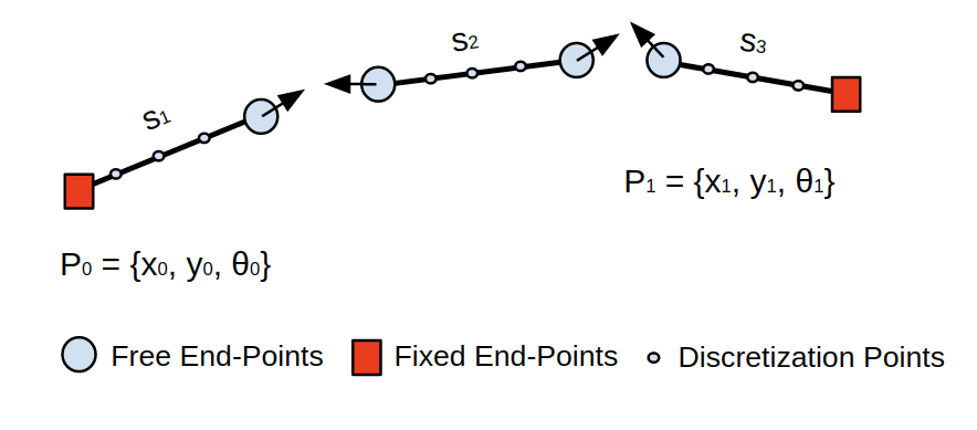
Inspired by the shape of R&S curves, we divide a whole parking maneuver into a minimum of three curve sections. Most of the trajectories that the R&S method produces consists of a maximum of four or five connected curves. Dividing a whole trajectory into three sections captures most of the solution families. In this proposal, we can imagine three separate vehicles trying to reach each other similar to the situation we see in a flag race (Figure 7).
Figure 7. Three separate curve sections on which each vehicle travels.
The three separate-curve-approach can be formulated with boundary conditions for each curve. The start and endpoint of the whole trajectory must be fixed. The curve connections (light blue circles) are the free boundary conditions for each of the curves that are needed to be connected by the optimization algorithm. In this way, we can obtain any arbitrary trajectory with cusps and breakpoints
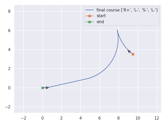
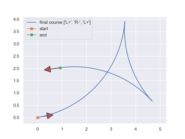
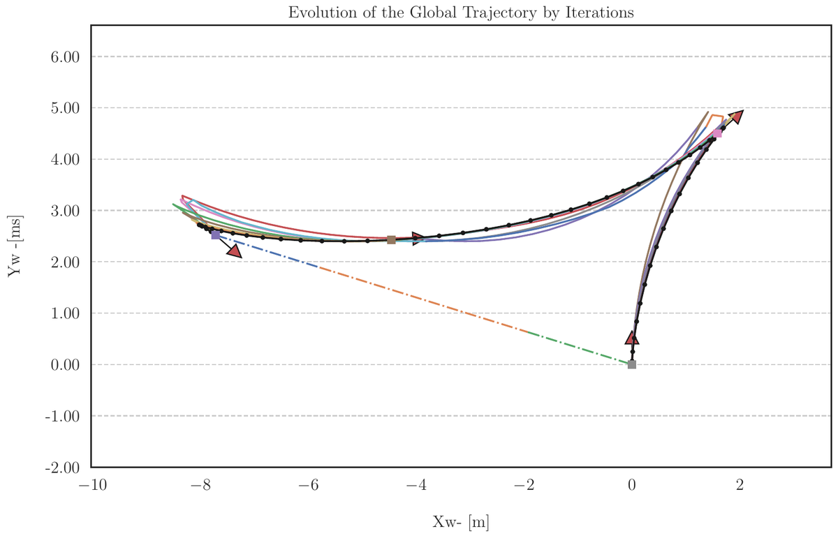
A solution to a nonholonomic motion planning problem without environmental constraints using the SCvx algorithm is shown in Figure 8.
Figure 8. A trajectory with two cusps solved by SCvx for an unconstrained case. The arrows with red-hats show the direction of the vehicle.
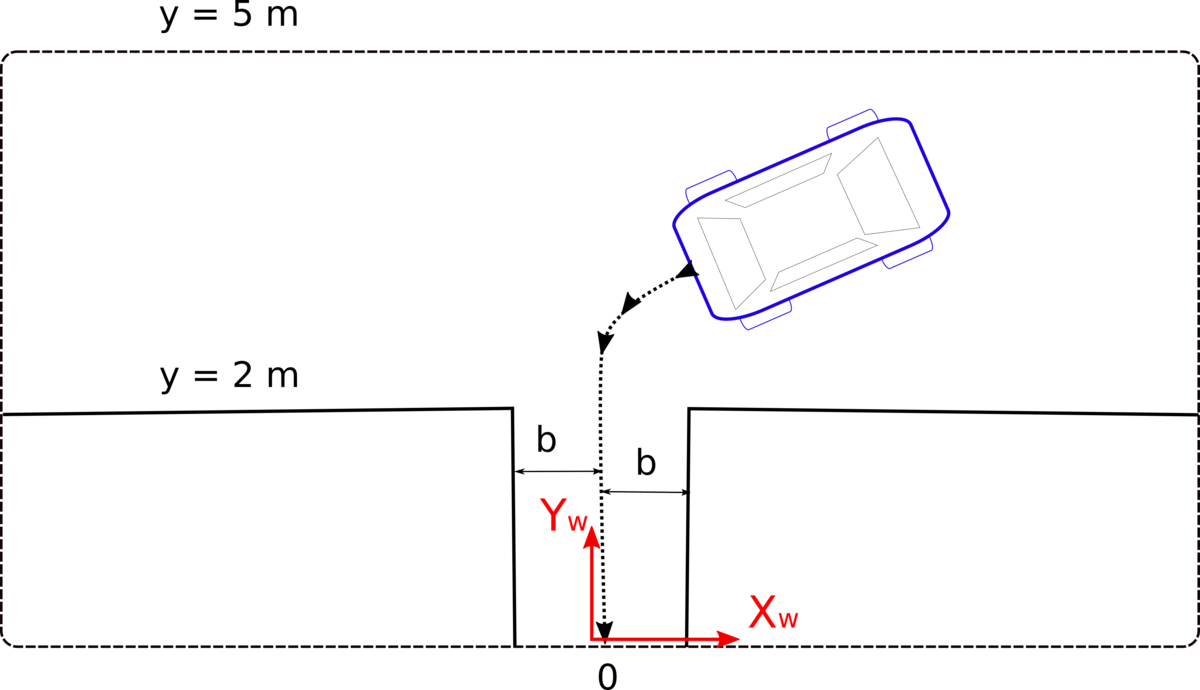
For the second issue; discontinuities in the environmental constraints, we used a state-triggered constraint formulation offered by the same authors of SCvx algorithms [5]. The authors formulate the keep-out zone for the spacecraft landing regions using the state-triggered constraints. The keep-out zone formulation resembles parking situations. In some optimization problems, we need to define the regions where some constraints could be active or inactive. This requires logical constraints or binary decisions such that, if some conditions occur, then some constraints are activated [if the triggering “condition < 0” ⇒ constraints < 0]. In mathematical optimization theory, these kinds of logical constraints are solved by mixed integer programming which is equally as hard as nonlinear optimization. We show an example of triggering and constraint conditions in Figure 9.
Figure 9. State-triggered constraint condition for a parking lot. Here the triggering conditions are xw < - b OR xw > b. When these conditions are triggered, the vehicle’s position value in yw direction must be yw>2 meters.
As you may notice, the solutions obtained at each iteration becomes an initial trajectory for the subsequent problem and hints us the regions where the logical constraints become active or inactive. This allows us to inject discontinuous environmental constraints when the iterated trajectory triggers the condition.
Using the state-triggers eliminates the use of complicated collision checking algorithms and alleviates the load of the solvers.
Complete Solution for Parking Maneuvers
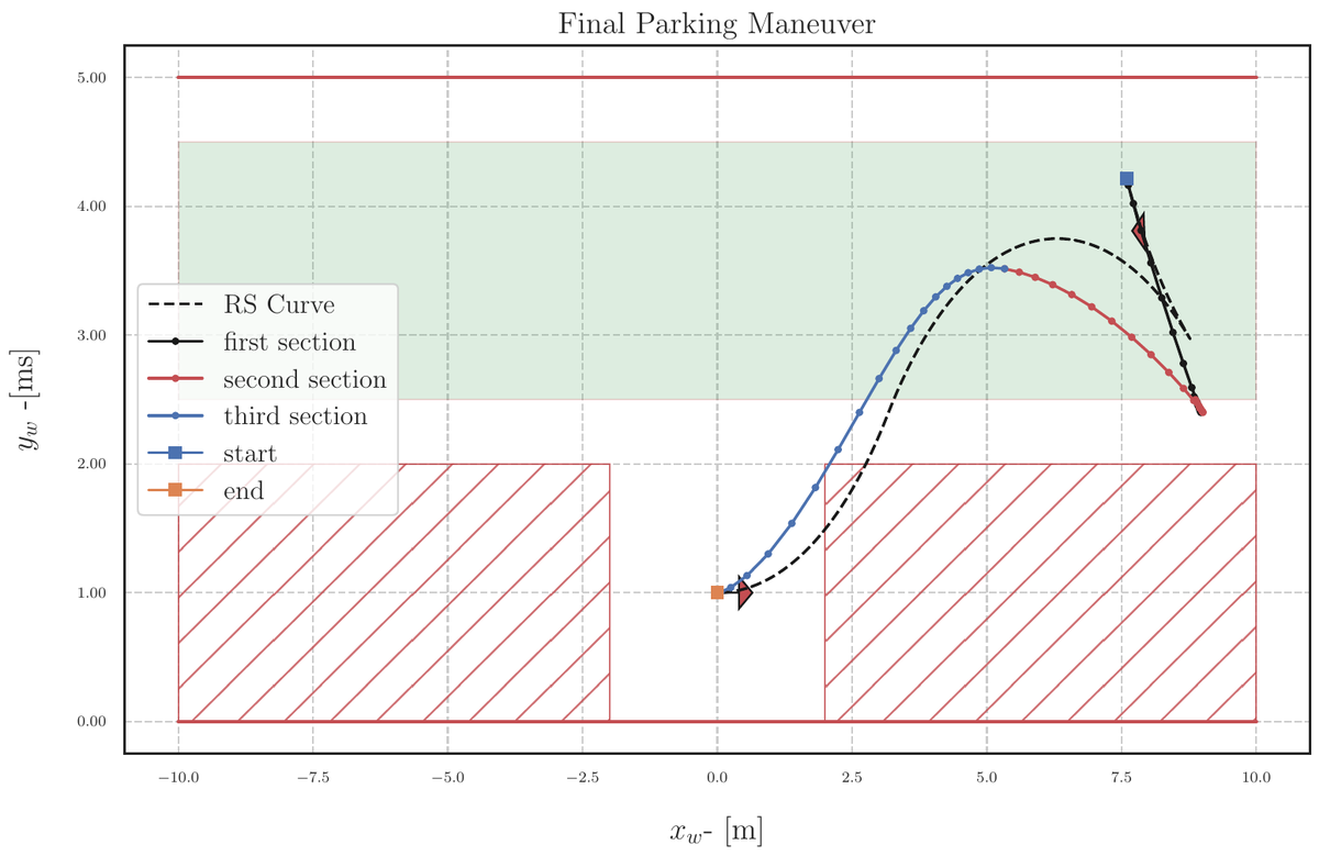
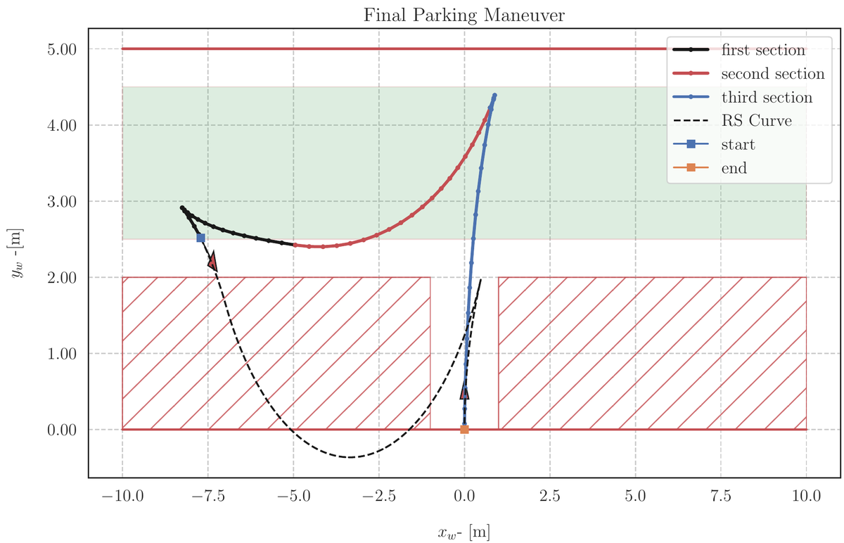
We applied the strategies we have mentioned to a couple of tight parking scenarios: parallel and perpendicular parking, which are shown in figures 10 and 11 respectively and with an animation in Figure 12. In these figures, we compare the SCvx solutions to the R&S curve solutions that are not aware of any constraints in the environment.
Figure 10. A parallel parking case. The vehicle starts in a random position and direction in the green shaded area and is requested to park in between two obstacles parallel to the X-axis.
Figure 11. A reverse parking case. The vehicle is requested to park perpendicular to the X-axis in between two obstacles.
Figure 12. An animation for a reverse parking maneuver.
Final Remarks
In this blog article, we summarized one of our publications presented at ITSC 2020; “Autonomous Parking by Successive Convexification and Compound State Triggers”. The detailed algorithms, equations and procedures and the related literature review and references can be found in our paper. We are planning to put the application of SCvx solutions into Autoware.
LaValle, S.M., 2006. Planning algorithms. Cambridge university press.
Boyali, A. and Thompson, S., 2020, September. Autonomous Parking by Successive Convexification and Compound State Triggers. In 2020 IEEE 23rd International Conference on Intelligent Transportation Systems (ITSC) (pp. 1-8). IEEE.
Mao, Y., Szmuk, M. and Açıkmeşe, B., 2016, December. Successive convexification of non-convex optimal control problems and its convergence properties. In 2016 IEEE 55th Conference on Decision and Control (CDC) (pp. 3636-3641). IEEE.
Szmuk, M., 2019. Successive Convexification & High-Performance Feedback Control for Agile Flight (Doctoral dissertation).


 , which means “the car must not be at the intersection until it is clear”. The paper proposes an efficient way to encode
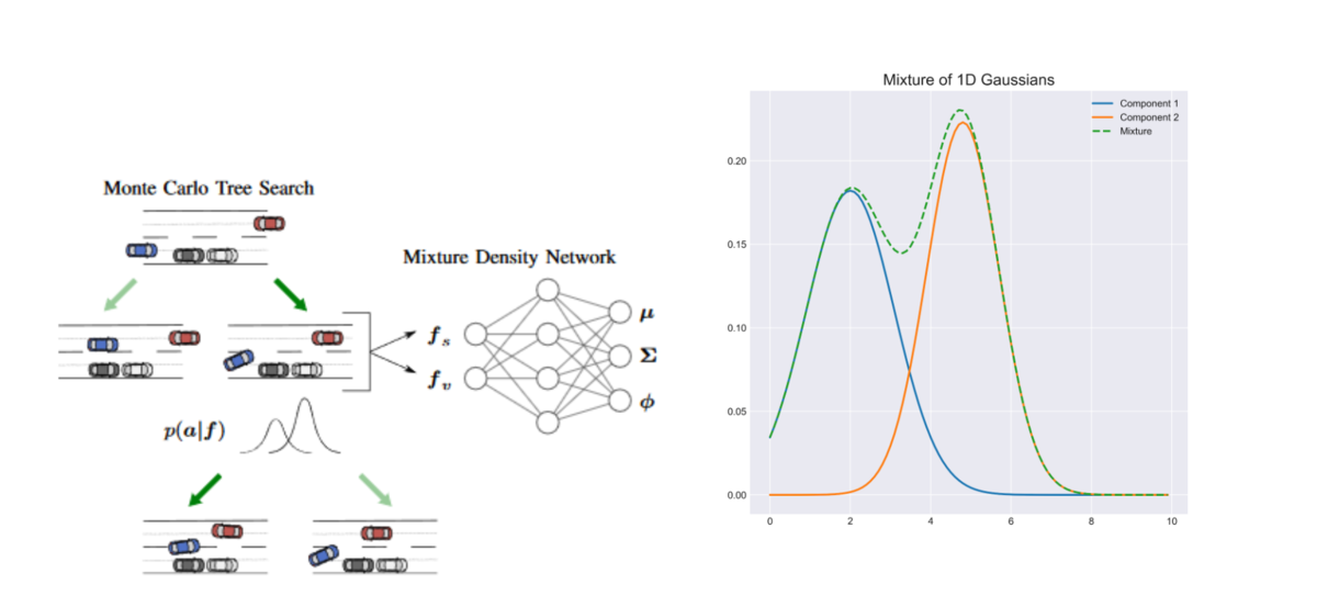


